Two numbers decide how good your RF measurement can ever be: how much of the signal bounces back, and how much of it disappears on the way through. Every adapter, cable, attenuator and termination on the bench is described by those two figures, and once you can read them you can predict a test setup’s error budget on paper before you connect anything.
This guide explains what VSWR and insertion loss actually measure, how to convert between the different ways vendors quote them, how to build a realistic loss budget, and where the two specifications quietly interact. It is written for engineers who already know what a 50 Ω system is, but who want to stop guessing when a datasheet says “VSWR 1.25:1 max” and “insertion loss 0.5 dB”.
What VSWR Actually Measures
VSWR — voltage standing wave ratio — is a scalar description of how badly a load is matched to a 50 Ω line. When a wave travelling down a coaxial line meets an impedance that is not exactly 50 Ω, part of it reflects. The forward and reflected waves add and subtract along the line, producing a standing pattern whose maximum and minimum voltages have a fixed ratio:
VSWR = Vmax / Vmin = (1 + |Γ|) / (1 − |Γ|)
where Γ is the reflection coefficient, Γ = (ZL − Z0) / (ZL + Z0). A perfect 50 Ω load reflects nothing, Γ = 0, and VSWR = 1.00:1. A short or an open reflects everything, |Γ| = 1, and VSWR is infinite.
Three practical consequences follow from that definition, and each one catches people out:
- VSWR is a magnitude, not a phase. A 1.5:1 load can be capacitive or inductive — VSWR cannot tell you which. If you need to know whether your mismatch will rotate into a problem at a specific frequency, you need a vector measurement (S11 with phase), not a VSWR number.
- VSWR is frequency-specific. A connector rated “1.25:1 max, DC–18 GHz” meets that limit across the band; the value at 2 GHz may be 1.05:1 and the value at 17.8 GHz may be 1.24:1. Always ask at which frequency the number applies, or whether it is a band maximum.
- VSWR is usually quoted as a maximum, not a typical. “1.3:1 max” is a production limit that every unit must meet. Typical units are often much better, but you cannot design a measurement uncertainty budget on a typical value.
You will meet VSWR everywhere in a coaxial catalogue: on 2.92mm precision adapters, on SMA fixed attenuators, on N-type coaxial loads. On all of them the number means the same thing: how much of the incident power fails to be absorbed.
Return Loss: The Same Mismatch, Expressed in dB
Return loss (RL) is the ratio of reflected power to incident power, written in decibels and given a positive sign by convention:
RL (dB) = −20 log10|Γ| = 10 log10(Pin / Preflected)
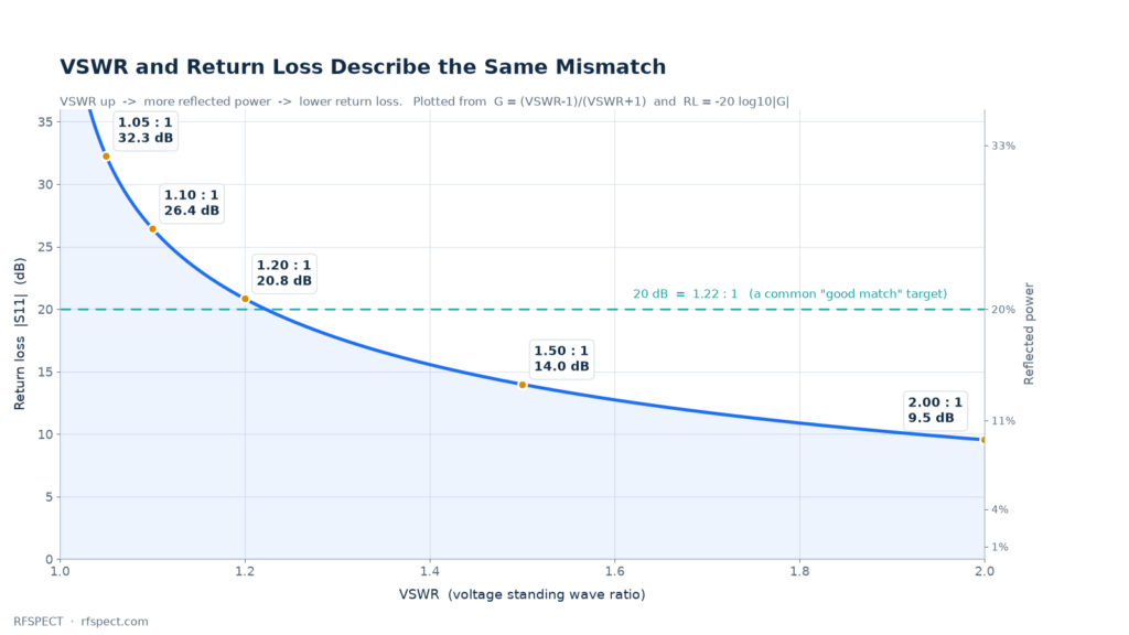
Higher is better. Return loss of 20 dB means 1 % of the power comes back; 10 dB means 10 % comes back. Network analysers display S11 in dB, so return loss is the natural unit inside a test lab, while VSWR remains the natural unit for component datasheets and for anything that has to survive a transmit path. Both describe one physical quantity, and the conversion is exact.
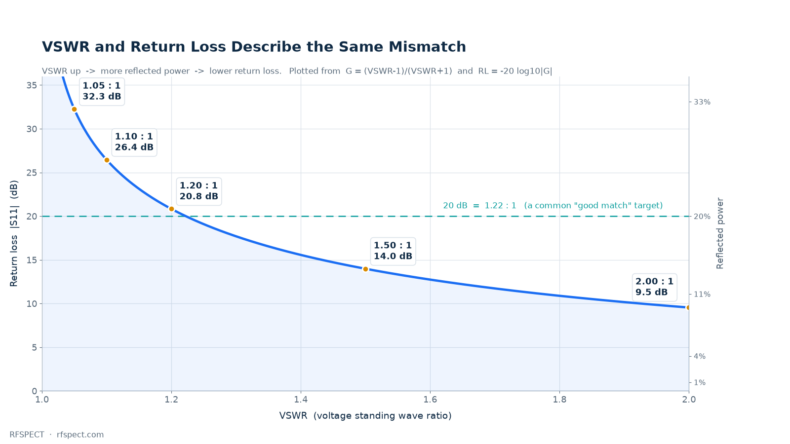
The table below covers the range most bench work lives in. Mismatch loss — the extra attenuation caused purely by the reflection — is included because it is the term people forget when they add up an error budget.
| VSWR | Return loss | Reflected power | Mismatch loss |
|---|---|---|---|
| 1.05 : 1 | 32.3 dB | 0.06 % | 0.003 dB |
| 1.10 : 1 | 26.4 dB | 0.23 % | 0.010 dB |
| 1.20 : 1 | 20.8 dB | 0.83 % | 0.036 dB |
| 1.30 : 1 | 17.7 dB | 1.69 % | 0.074 dB |
| 1.50 : 1 | 14.0 dB | 4.00 % | 0.177 dB |
| 2.00 : 1 | 9.5 dB | 11.1 % | 0.512 dB |
One reading of that table is worth memorising: 20 dB return loss is a good match, 10 dB is a mediocre one, and the difference in mismatch loss between them is only 0.5 dB. That is why a 1.5:1 component rarely ruins a system that has 3 dB of margin, and why chasing 1.02:1 is usually a waste of money unless the reflection itself is the measurand.
Insertion Loss: What Is Really Inside the Number
Insertion loss is the drop in transmitted power when a device is inserted into an otherwise matched line: IL (dB) = 10 log10(Pin / Pout), measured with both ports terminated in 50 Ω. For a cable assembly, that single figure hides three contributions:
- Dielectric loss — absorption in the PTFE, FEP or foam insulation, roughly proportional to frequency.
- Conductor loss — resistive loss in the centre conductor and shield, which grows with √f because of skin effect. In a well-made cable this dominates above a few hundred MHz.
- Connector and launch loss — typically 0.05–0.2 dB per interface, plus a small mismatch contribution that appears as ripple rather than as a smooth slope.

Two rules cover most estimates you will ever need:
- Loss scales with √f. If a cable loses 1.0 dB at 4 GHz, it loses about 2.1 dB at 18 GHz and 3.2 dB at 40 GHz. Vendors quote loss at one or two frequencies for exactly this reason.
- Loss scales linearly with length. Double the cable, double the loss. Half the length, half the loss. There is no “free” bend radius that recovers it.
The practical trap is comparing a thin flexible cable with a low-loss cable of the same connector type. A 2.5 mm RG316 assembly and a 2.4 mm phase-stable test cable share almost the same outside diameter, yet differ by more than 2:1 in loss at 18 GHz, because one uses solid PTFE and the other a low-density dielectric with a larger centre conductor. When a measurement looks 1.5 dB worse than expected at millimetre-wave frequencies, the cable — not the instrument — is usually the reason. Our cable assembly and coaxial cable ranges list loss per metre at 1, 6, 18 and 40 GHz so this comparison can be made before ordering.
Building a Loss Budget: A Worked Example
Take a typical 18 GHz bench measurement: a signal generator, a 1 m low-loss test cable to the DUT, one adapter at the DUT, and a power sensor on the other side. Sum the contributions instead of guessing:
| Element | Typical loss at 18 GHz | Note |
|---|---|---|
| 1 m 2.4 mm phase-stable cable | 1.3 dB | √f law, length-dependent |
| 2 × cable connectors (already included) | included | launch loss is part of the assembly spec |
| 2.92mm male to SMA male adapter | 0.15 dB | precision grade, 1.15:1 typ. |
| 2.92mm 10 dB / 10 W attenuator | 10.2 dB | nominal value plus 0.2 dB excess loss |
| Mismatch loss (source 1.3:1, load 1.2:1) | 0.04 dB | usually negligible below 26 GHz |
| Total | ≈ 11.7 dB | budget ±0.6 dB for uncertainty |
That total is what you subtract when you calculate the power actually reaching the DUT. Skip it and a 10 dB attenuator “measures” 10.4 dB — a 4 % error that nobody notices until a link budget fails in the field.
Where the Two Specifications Interact
VSWR and insertion loss are usually specified separately, but in a real measurement chain they combine into something neither number shows alone: mismatch uncertainty. When a source with reflection Γ1 looks into a load with reflection Γ2, the power delivered can vary by
±20 log10(1 ± |Γ1|·|Γ2|) dB
With two 1.5:1 interfaces (|Γ| ≈ 0.2 each) that is ±0.35 dB of pure uncertainty — larger than the mismatch loss itself. Add a third mismatched element and the ripple grows. This is the real reason precision adapters exist: not because 0.1 dB of extra loss matters, but because a 1.05:1 interface instead of a 1.5:1 one cuts measurement uncertainty by a factor of four at millimetre-wave frequencies. It is also why the choice of connector interface changes the quality of a measurement chain before any cable is attached.
The ripple carries information too. The spacing between successive peaks in an insertion-loss sweep equals c / (2·L·√εr) for a cable of length L, so a periodic ripple in a loss trace is a distance-to-fault measurement in disguise. A smooth slope is absorption; a periodic ripple is a reflection from a connector, an adapter or a damaged cable.
Reading the Datasheet: Five Checks
- Max or typical? Design with the max; use the typical only to predict what you will usually see.
- At which frequency? A single VSWR number without a frequency range is marketing; a band maximum is a specification.
- dB or dB/m? Cable loss is per unit length; assembly loss is total. Mixing the two produces errors of a factor of three or more.
- Included or excluded connectors? Some vendors quote cable-only loss and add connector loss separately.
- Temperature and power? Loss rises a few percent between 25 °C and 85 °C, and high-power terminations derate with ambient temperature. Our 2.92mm 15 W termination, for example, is rated at 25 °C and must be derated above it.
Which Number to Care About
| Task | Dominant specification | Why |
|---|---|---|
| Transmit path, power handling | VSWR / return loss | Reflected power heats the source and raises voltage stress |
| Receiver sensitivity, long cable run | Insertion loss | Loss directly subtracts from the signal budget |
| VNA calibration and S-parameter accuracy | Both, plus phase stability | Mismatch uncertainty dominates the error term |
| Power measurement | Insertion loss + mismatch loss | Both shift the reading by a few tenths of a dB |
| Filter and antenna test | Return loss in band edges | VSWR spikes identify resonances and detuning |
FAQ
Is 1.5:1 VSWR good?
For a general-purpose component, yes — 14 dB return loss reflects 4 % of the power and costs only 0.18 dB of mismatch loss. For a metrology-grade adapter or a calibration standard, no: precision interfaces are specified at 1.05:1 to 1.15:1 because mismatch uncertainty, not loss, is the limiting error.
Why does my cable measure worse than its datasheet?
Three usual causes: the datasheet quoted cable-only loss while you measured an assembly including connectors; you measured at a higher frequency than the quoted point; or the cable has a damaged connector or a tight bend. A periodic ripple in the sweep points to a reflection, a uniformly higher slope points to length or temperature. If the interface in question is a 1.0 mm or 1.85 mm air line, handling is the more likely cause — the 1.0 mm connector care guide shows what torque, cleaning and a worn mating plane each do to the trace.
Can I convert VSWR to return loss without a chart?
Yes. Compute Γ = (VSWR − 1)/(VSWR + 1), then RL = −20 log10|Γ|. For a quick mental check, remember the ladder: 2.0:1 = 9.5 dB, 1.5:1 = 14 dB, 1.33:1 = 17 dB, 1.2:1 = 21 dB, 1.1:1 = 26 dB. The closer you get to 1.0:1, the faster the return loss climbs.
Does a 3 dB attenuator add 3 dB of insertion loss?
Almost. A real 3 dB pad shows 3.1–3.3 dB at DC and a little more at high frequency, because the resistive elements have parasitic reactance. The excess loss is quoted in the datasheet as a maximum over the band.
What insertion loss should I expect at 40 GHz?
A 1 m low-loss 2.4 mm assembly lands around 2 dB; an RG316 assembly of the same length reaches 4 dB or more. Above 40 GHz, the connector interface and the cable’s mode suppression usually matter more than the dielectric itself.
Does VSWR affect insertion loss?
Only through mismatch loss, which is small: 0.5 dB even at 2.0:1. What VSWR really affects is the repeatability of a measurement, because small changes in the reflection rotate into different readings each time you reconnect.
The Short Version
VSWR and return loss describe the same reflection; use return loss for analysis and VSWR for specification. Insertion loss is a sum of dielectric, conductor and connector contributions that grows as √f and scales with length. Budget both before you build a setup, allow a few tenths of a dB for mismatch uncertainty, and buy precision interfaces when repeatability matters more than cost — the loss itself is rarely the problem.
If you are still choosing an interface for a new setup, start with the RF adapter overview and the interface comparison guide; if the numbers above look familiar but your budget does not close, send us the frequencies and lengths and we will check the loss budget against real measured data.
About the author — this guide is maintained by the RFSPECT engineering team in Shenzhen, who design and test coaxial adapters, attenuators, terminations and cable assemblies to 110 GHz. If a number here disagrees with the drawing you received, tell us and we will correct it.